Adaptive Hierarchical Encoding in Model
Neurons and H1
Erik Flister, Emily Anderson
June 2006
Abstract
We propose a novel experiment design to
investigate stimulus encoding and adaptation in sensory neurons. Neurons are exposed to repeated trials
of a nearly identical time-varying stimulus. The stimulus is divided into three sections, the first and
third of which never vary. The
first stimulus section serves to reset the neuron into an identical adaptive
state across trials. The stimulus
is modified systematically for the middle section of each trial, revealing how
small stimulus changes are reflected in the spike timing of the neural
response. Due to differential
adaptation during this middle section, responses to the identical final section
vary, reflecting their context-dependence. Our stimulus design exposes the decaying time dynamics of
this memory effect. We demonstrate
the design in model neurons and the motion-sensitive H1 fly neuron, revealing
adaptation to stimulus variance ("contrast") in both cases. Our key novel theoretical contributions
are 1) that features are encoded by spike "swoops" that respect
temporal boundaries between features, 2) that this pattern holds for
sub-features within features, forming a fractal pattern so that encoding is
hierarchical, 3) that spike times within a single trial correspond to stimulus
features at varying, rather than consistent, latency, 4) that refractory
effects serve to delay, rather than prevent, future spikes, and 5) refractory
effects play an important role in very short-term adaptation.
Introduction
Spike
times in sensory neurons across phylogeny, from the periphery to high-order
cortices, have proven to encode dynamic stimuli that contain suitably high
frequencies with reliability and precision (Mainen and Sejnowski). The classic experiment that demonstrates
this is to repeat the same stimulus over many trials while recording the spike
times of the neural response. The
peri-stimulus time histogram (PSTH) describes the observed probability of
spiking at each time following stimulus onset across the trials, and typically
comprises discrete "events" during which the neuron fires at most
once; this property is known as "sparse" encoding. Measures of the event widths (typically
the variances of fitted Gaussians) indicate the temporal precision of spike
times, while their integral indicates the event reliability, the probability
that any given response will spike during the event.
Sensory
neurons are also frequently found to adapt, which means that their encoding
scheme is context sensitive, so that they encode identical stimuli differently
depending on the recent stimulus history.
Adaptation may have the teleological purpose of improving efficiency,
the number of spikes required to encode a fixed amount of information about the
stimulus. Sensory neurons often
respond only to changes in stimuli, which avoids costs associated with using
spikes to encode static stimuli.
This could be compared to a common form of video compression designed
for efficient transmission of "talking head" scenes that involve very
little motion; since frame-to-frame differences are small, it is more efficient
to assume a static scene and only represent violations of this assumption than
to represent time-varying luminance directly. This is one form of adaptation, since the same absolute
stimulus may evoke a large response if it is different from preceding stimuli,
while evoking only a baseline response when there is no change. Adaptation of this kind could be
explained as a non-adaptive response that simply encodes the time-derivative of
the stimulus, rather than the stimulus itself.
Another
form of adaptation is a tuning of the response to maximize dynamic range, given
the range of values recently occupied by the stimulus. Contrast adaptation in the visual
system is an example of this; stimulus encoding is relatively insensitive to
contrast. That is, when luminances
have been within a small range for a while (low contrast), visual neurons
adjust so that they encode contrast-independent scene information (edge
locations, for example) in about the same way as when luminances vary across a
wider range (high contrast). For a
short time after contrast suddenly changes, neurons will encode the same
stimulus differently (at lower efficiency, less information per spike), because
they have not yet had time to adapt to the new contrast regime and adjust their
dynamic range to match the signal content (Denning and Reinagel).
Reverse
correlation techniques are often used to more or less accurately recover the
function that describes how sensory neurons encode stimuli in spike times (first-
(spike-triggered averaging) and second-order (spike-triggered covariance)
Wiener-kernel methods, Bialek).
This approach is often successful for recovering the encoding function
over small time scales, and usually reveals the differentiating-filter (high-pass)
properties of sensory neurons. But
stimulus dimensionality over the long time scales associated with other forms
of adaptation is often too large to allow adequate sampling. Moreover, most reverse correlation
techniques (all except "maximally informative dimensions" (Sharpee))
only work for Gaussian stimuli; since natural stimuli are not typically
Gaussian, such techniques are limited to studying neural response to stimuli
with unnatural 3rd- and higher-order moments (spectral frequency content, the
second moment, can be matched to that of natural stimuli, but higher order
moments are uniquely constrained by the first two moments for Gaussian
processes). Thus, slow adaptation
dynamics, especially in the natural stimulus regimes that sensory neurons are
presumably phylo- and ontogenetically optimized to represent, are not easily
probed.
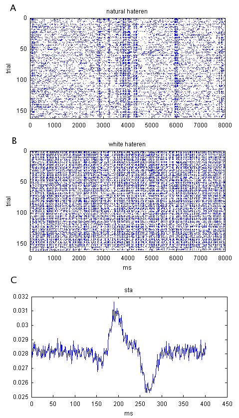
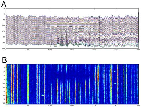
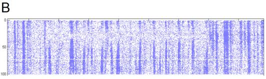
Figure
1. Example raster plots demonstrate
spike time precision and reliability.
These data were recorded by Erik Flister in Pam Reinagel's lab. They are from an LGN neuron recorded
via a chronic tetrode microdrive implant in an awake behaving rat. The stimulus was time-varying
full-field luminance. In one case
(B),
the stimulus was Gaussian and contained no temporal correlations
("white"), while in another (A), it was drawn from a single pixel of a
monochromatic movie shot at human eye-level while walking through a forest
during daylight (van Hateren). Raster
plots separate trials vertically and show spike times as dots, positioned
horizontally according to when they occurred relative to the stimulus. Also shown (C) is the spike-triggered
average stimulus (the average stimulus that preceded a spike in the white
dataset), which represents the best single linear filter approximation of the
cell's stimulus-to-spike transfer function.
Experimental
Design
We
designed a novel experimental paradigm to reveal qualitative features of spike
time encoding and adaptation. Real
and model neurons are presented with repeated trials of identical noise
stimuli, using a waveform produced by some stochastic process. During a middle section of the
stimulus, a parameter is varied by small amounts across trials, but the
stimulus is identical for the first and final sections. The first section serves to replicate
the results discussed above; the responses to these identical stimuli should be
reliable and precise across trials and demonstrate the stationarity of the
neuron's behavior. This section
also serves to equalize the neuron's adaptive state; it should be longer than
the neuron's memory, so that by the end the neuron always responds the same
way. During the middle section,
the original waveform is modified by small steps in some systematic way. The neural response should demonstrate
how the neuron encodes small changes in the varied parameter when it is in the
adaptive state induced by the first section of the stimulus. During the final section, the stimulus
is again identical across trials.
If the neuron were in a constant adaptive state during this section, its
response would be reliable and precise, as it was in the first section. However, to the extent that the
parameter variations in the middle section change the adaptive state of the
neuron, its response to the final section will show context dependence. As the neuron "forgets" about
the middle section of stimulus, this context dependence will disappear, so the
variations in response to the last section should reveal the time dynamics of
adaptation.
Here
it is important to point out that, in the case of in vivo recording, we are
recording from a single neuron whose activity is a measure of the activity of
the whole neural network presynaptic to it; thus its "memory" may be
much longer than is possible for a single neuron in isolation.
The
parameter we vary is the noise variance (also called amplitude or
contrast). We achieve this by
simply multiplying the middle section of the waveform by a constant. We slowly vary the magnitude of this
constant from negative to positive values across trials (ideally the values
would be shuffled over trials so that the results will not be confounded by
non-stationarities such as subtle electrode drift or diminishing health of the
preparation, although we did not shuffle here). Many other parameters could be gradually varied instead: the waveform could be shifted, expanded
or compressed in time, its mean could be shifted, it could be filtered for
frequency content, or sections could be silenced, to give just a few examples
we are interested in. For the
model neurons, the stimulus was injected current. For H1, a motion sensitive neuron in the early fly visual
system, the stimulus was the horizontal position or velocity of a spatially
varying luminosity pattern. But in
principle any physical quantity within the receptive field of a sensory neuron
could be driven in this way: full
field luminance (vision), vibration (somatosensation), sound-pressure level
(audition), and so on. In order to
probe H1 as closely as possible to its natural operating regime, our spatial
pattern consisted of Gaussian noise filtered to enjoy a "natural" 1/f
spectrum, as did our velocity and position profiles, and current injection in
the case of the model.
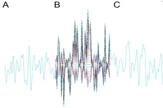
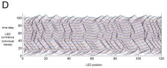
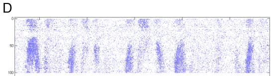
Figure
2. Stimulus. Our example stimulus is 1/f Gaussian
noise, divided into three sections.
The first and final section (A, C) are always identical across trials. The middle section (B) is multiplied by a
constant that slowly varies from a negative to a positive value over trials,
thus altering the stimulus variance (equivalently, "amplitude" or
"contrast") during that section and reversing the waveform
polarity. These waveforms are used
to drive current injected into model cells or the position or velocity of a
spatial pattern for H1 (D).
Results
The
model cells we used were the Izhikevich model (Izhikevich), an extremely
efficient 2-dimensional dynamical model with 4 parameters that allows very
close quantitative approximation to the physiological behavior of a wide
variety of known cell types. Given
the intriguing nature of the results, it would be interesting to check the
response of simpler models, including integrate-and-fire,
quadratic-integrate-and-fire, and inhomogeneous Poisson and gamma
point-processes with rate governed by a thresholded linear filter
(linear-nonlinear-Poisson (LNP) and -gamma LNG models). Much of the dynamical model response
appears to involve refractory-like effects, which will not be captured by any
of these simpler models except LNG, and positive feedback, not captured by any
except quadratic-integrate-and-fire.
We would also like to test map-based models, which do capture positive
feedback and refractoriness (Timofeev).
The
key observation in the model response is the hierarchical reverse-J
structure. This stimulus paradigm
allows, for the first time, the identification of single spike events that
correspond to the same feature across trials, even though the spike itself
occurs at widely disparate times.
As features in the stimulus waveform become large enough to be resolved
by the neuron (cross threshold), they first cause spikes with high latency --
it has long been known that low-contrast stimuli are processed with higher
latency by sensory neurons. As the
feature becomes larger, it causes a faster depolarization, which causes the
positive feedback chain-reaction of sodium-channel activation that underlies a
spike to occur with lower latency.
Thus, the spike time asymptotes quickly from its initial high latency to
a fixed, short latency with respect to the feature. We will refer to the resulting single-spike reverse-J
structure across trials as a "swoop." Then, as additional details of the feature become resolved,
more spikes follow the same pattern, swooping in behind the original
spike. A key point revealed here
is that, in any one trial, individual spikes are occurring with dramatically
different latencies. This insight,
presented here for the first time, flies in the face of typical
reverse-correlation analyses, which explicitly assume that each spike encodes
stimulus information at a consistent relative time-lag.
A
second key point, also novel, is the hierarchical nature of the encoding. As features grow in strength,
additional spikes swoop in behind the initial ones, occurring first with high
latency and then with low latency, joining together to form low-latency bursts
that represent the features.
Intriguingly, temporal (vertical) boundaries between features are
respected -- "swoops" from adjacent features never overlap. This pattern holds for sub-features
within features, resulting in a hierarchical fractal-like pattern.
Refractory
effects played an important role in the response, particularly when a weak
feature was followed by a stronger feature. Since the strong feature becomes resolved first, some of its
spikes are established by the time the weaker feature's spikes appear. When they do, their refractory effect
delays, but never prevents, the subsequent features' spikes. This effect seems to preferentially
affect spikes that have not yet asymptoted; well-established low-latency spikes
are not perturbed, but the effect can actually jump over them to affect
subsequent nascent spikes. This
refractory effect appears to play the majority role in adaptation effects for
this single-neuron model.
Prior
to seeing the model response, we expected spike bifurcations to play a much
larger role. Bifurcations occur,
but are relatively rare.
Figure
3. Model response reveals variable-latency
hierarchical encoding and refractory effects that can delay, but not prevent,
subsequent spikes.
The
horizontal time scale measures half milliseconds.
A A single swoop is highlighted.
B Hierarchical secondary-swoops that join
together to form a low-latency burst are highlighted.
C Vertical boundaries that separate
features are shown.
D Refractory effects delay, but do not
prevent, subsequent spikes as preceding features become resolved. This effect is absent for
well-established low-latency spikes, and can even transfer to spikes that
follow them.
E Refractory effects play a role in
adaptation.
F A rare spike bifurcation.
For
the in vivo
H1 experiments, our stimulation equipment did not allow precise temporal
control below about 10ms, and likely could not adequately simulate smooth
motion, although we were able to prevent the disaster of jitter accumulation
(see Methods). Despite the limitations, our results
confirmed the model predictions of asymptoting latency, hierarchical
fractal-like encoding, and did exhibit adaptation. These promising preliminary results encourage a system
upgrade to investigate at high precision whether the fine temporal features of
our model predictions hold at a precise spike-timing level in vivo.
During
the variable part of the stimulus, spike events asymptoted from high to low
latency and exhibited the same hierarchical swooping behavior as the
model. During the adaptive
portion, when the stimulus was identical but context varied, the neural
response showed adaptive trends that depended on context. The most obvious adaptive feature was a
large increase in spike rate in response to the same stimulus intensity when it
was preceded by lower stimulus intensity.
This was even more apparent at the beginning of trials, which was
preceded by an inter-trial interval of around 30s of darkness.
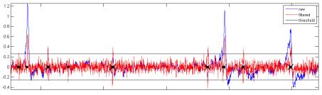
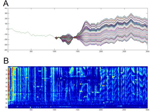
Figure
4. Physiology. Extracellular potential was recorded at
20 or 30kHz (blue)
from an isolated physiology amplifier configured to pass 300Hz-10kHz at
10,000X, and filtered (red) using an optimal zero-phase 60th-order FIR
filter designed by Matlab's fir1() to have a pass-band from 5-99% of the
Nyquist frequency. Spike times (black
markers)
were identified by upward-going threshold crossings at 3.5 times the standard
deviation of the filtered signal (black).
Note that this spike detection algorithm turned out to be terrible; it
catches multiple threshold crossings per spike, so the threshold should be much
higher and single-sided.
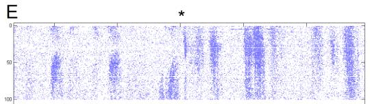
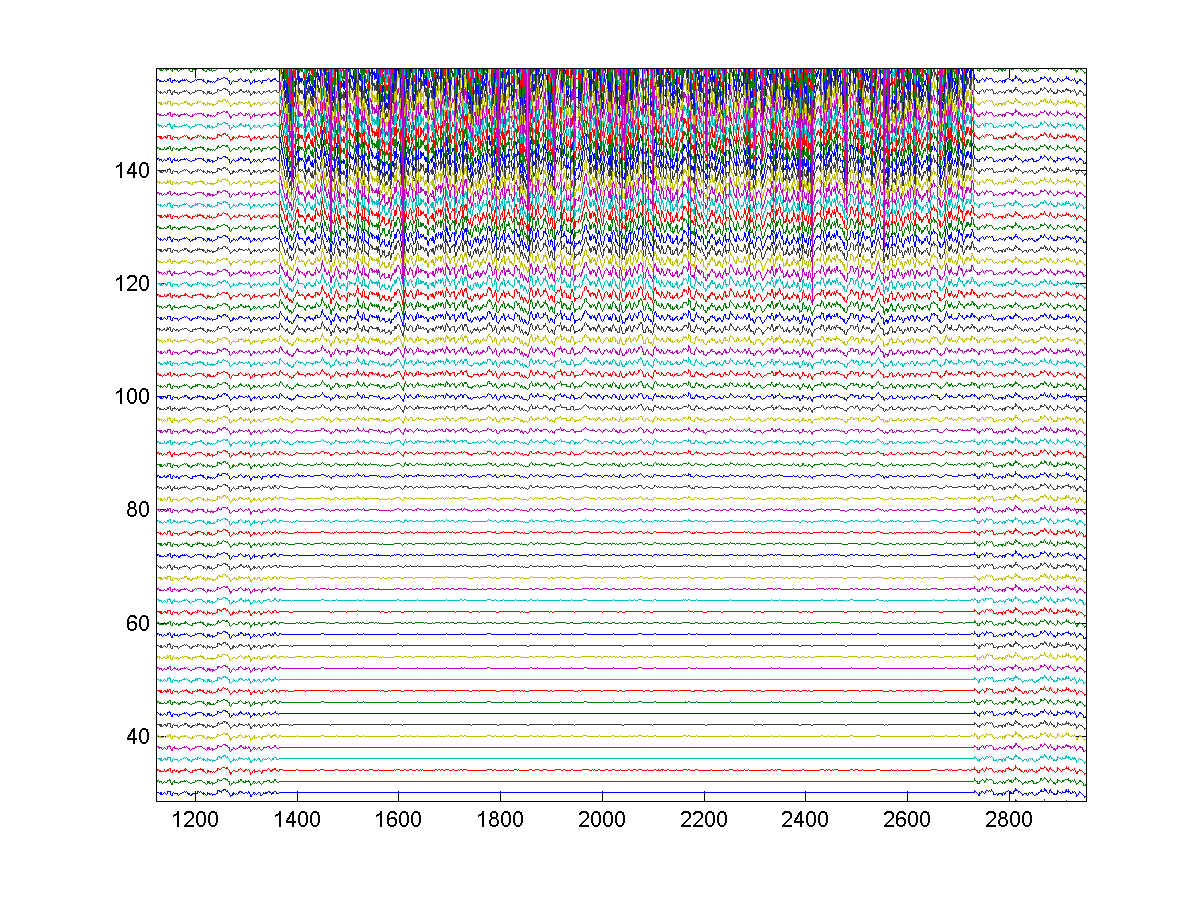
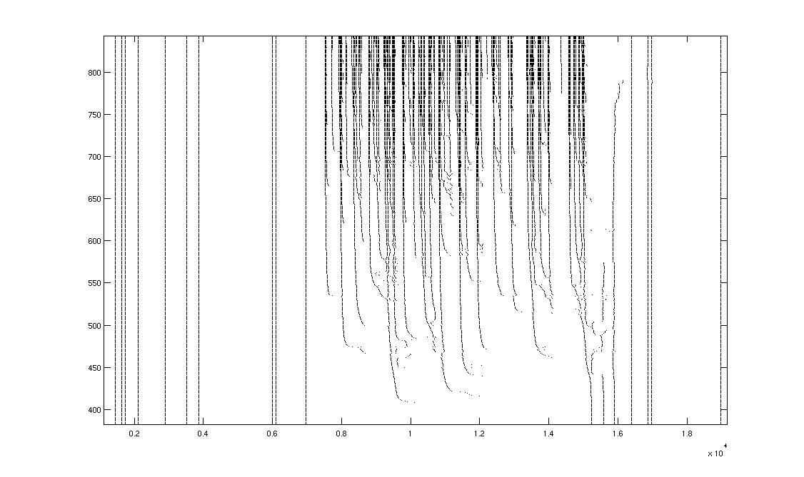
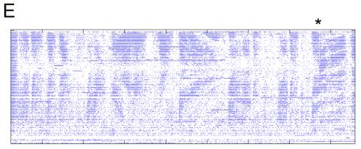
Figure
5. H1 position response.
100 trials. An entire trial contains 3000 frames
and lasts a little less than 60s.
The zero-motion trial was around trial 30.
A Spatial pattern position varied across
trials.
B Spike rate response is shown in pseudo-color,
lightly smoothed with a 2-D Gaussian filter. The top 2% of rates, which corresponded to artifacts from episodes
of fly motion, are clipped, to improve dynamic range. Non-stationarity across the experiment is clearly visible;
the cell became better isolated and responded more strongly to the beginning of
trials as the experiment progressed.
C Raster of actual spike times.
D Detail on variable period shows spike
events asymptoting in different directions and hierarchical fractal swooping.
E Detail of transition from variable to
adaptive portions of response.
Approximate location of transition (*). During the adaptation period, increased
response to identical stimuli when preceded by low-velocity stimuli is
visible. This is also visible in B as the high rates that
follow the ~30s inter-trial dark interval.
When
the stimulus parameter is velocity, the stimulus waveform must be integrated to
recover position. Since the
initial position was always the same, the middle section of varying velocity
causes the positions to diverge from trial to trial, so that in the final
section, pattern velocity is conserved but stimuli are not identical because
position is offset. H1 response
reflected positional offset, probably because the offset moved features used
for motion estimation into and out of its receptive field. A better future design for
investigating adaptation would be to offset the positions at the beginning of the
trials so that the varying velocity section will cause them to exactly align
for the final section. It is not
possible to merely reverse the velocity waveforms because time-reversal does
not conserve the phase spectrum.
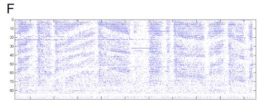
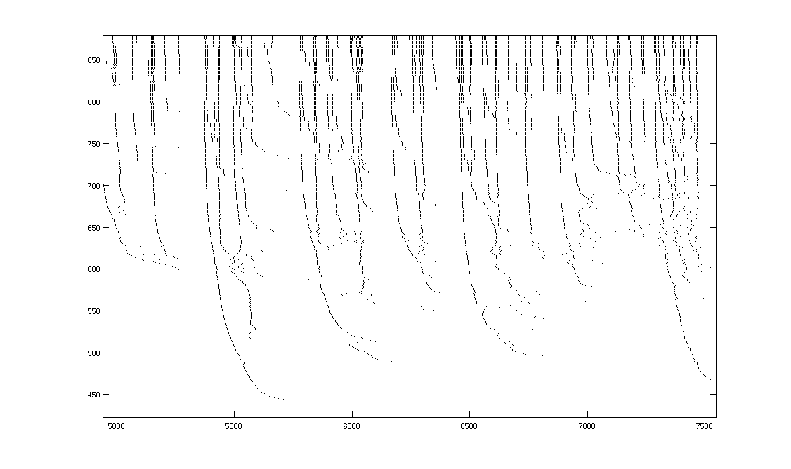
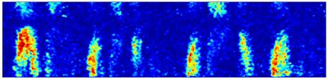
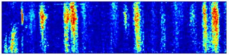
Figure
6. H1 velocity response.
100 trials. An entire trial contains 3000 frames
and lasts a little less than 60s.
The zero-motion trial was around trial 30.
A Spatial pattern velocity varied across
trials according to a waveform similar to that in 2A. When driving pattern velocity, the
stimulus waveform must be integrated to recover position. Since the initial position is always
the same, the middle section of varying velocity causes the positions to
diverge from trial to trial, so that in the final section, pattern velocity is
conserved but stimuli are not identical because position is offset.
B Spike rate response as in 5B.
C Raster. The cell was lost for the final few trials (*). Spontaneous activity in the dark can be
seen during the beginning of the inter-trial interval (o). H1 response reflected positional
offset, probably because the offset moved features used for motion estimation
into and out of its receptive field.
D
E Detail of transition from variable to
adaptive portions of response.
Approximate location of transition (*). Dark streaks are fly motion artifacts.
F Detail of the adaptive portion of
response. Tracking of position
offset is clearly visible as chevrons.
Methods
Female
flies (the male fly visual system is more designed for pursuit of small dark
objects against a bright background, and does not give good full-field motion
response) were dissected as previously described (Tumer) and placed near the
center of an arena surrounded by 96 columns of LEDs, which spanned 3 degrees of
horizontal visual field each. A
96-channel digital I/O National Instruments card, the PC-DIO-96, tells each
column of LEDs whether it should be set to a high or low luminance, while an analog
card sets the actual value for the high and low luminances.
Evren
Tumer wrote a LabView program ("/Seth Brundle/the_fly5.vi") that can
present rotating patterns described by two luminance values. Unfortunately, he found that the 3
degrees spanned by the LEDs were within the spatial resolution of the fly
visual system, so that H1 responds as if it is seeing the individual discrete
jumps as the pattern moves across LEDs, rather than smooth motion (the neural
response is simply a burst of spikes each time the pattern moves by one
LED). His software also does not
allow the arbitrary definition of stimulus waveforms, as required by our
experimental design. He has another
LabView program ("/Seth Brundle/newfly.vi"), that does allow arbitrary
definition of time-varying full-field luminance, but it did not produce the
expected results when we tried it.
Therefore, we decided to write our own stimulus presentation software,
but the_fly5.vi is convenient for locating and isolating H1.
To
overcome the resolution problem, we do not restrict the spatial pattern to two
luminance values, but discretize an arbitrary waveform into n luminance values
(n=10 for our experiments).
Because higher n reduces the presence of hard edges in the stimulus and
prevents boundaries between luminance values from shifting on the same
"frame," this approach provides a closer approximation to smooth
motion for a fixed spatial resolution.
The values are gamma-corrected and each frame in the stimulus is created
by interlacing n "sub-frames," each of which lights up the
appropriate LEDs at its gamma-corrected luminance value. This has two deleterious effects. It reduces temporal resolution by a
factor of n, and since each LED is on for only one of n sub-frames, overall
luminance and contrast are drastically reduced. A future improvement would be to choose the n luminance
values dynamically, optimally distributing them to the values actually
requested frame-by-frame, rather than statically allocating them uniformly over
the full range of possible values.
We did not have time to assess whether the waveform discritization
approach created an adequate approximation to smooth motion; the data we
recorded could be analyzed to reveal whether bursts of spikes merely followed
frame or sub-frame transitions.
The results were subjectively smoother than the 2-luminance value
approach, but close examination of a spike raster reveals regularly spaced
bursts of spikes, suggesting that the motion is still too coarse. But this could also be an artifact of
the poor spike-detection algorithm that is triggered by multiple threshold
crossings per actual spike.

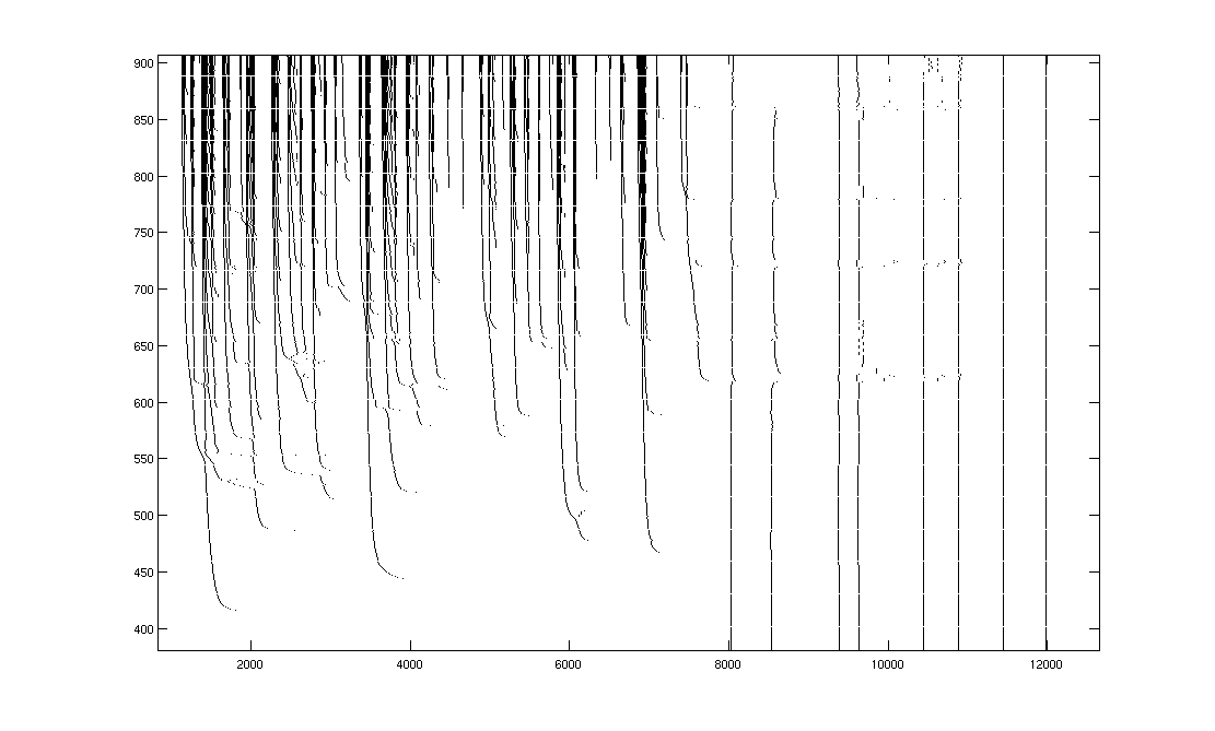
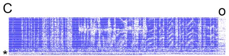
Figure
7. Regularly spaced bursts of spikes
suggest the discretized stimulus is not encoded the same way that continuous
motion would be, but this may be an artifact of multiple spike-detections per
actual spike.
We
first tried using Matlab's Data Acquisition toolbox, which provides commands
for controlling the National Instruments cards that drive the LEDs. We found that execution timing in
Matlab, even when compiled into a function rather than interpreted in a script
file, is too slow and variable for our high frequency and precision
requirements (minimum line execution time is ~10ms). We then tried using Matlab's loadlibrary()/calllib()
commands to access the c API for the cards directly ("traditional
NI-DAQ," available on the National Instruments website at
ftp://ftp.ni.com/support/daq/pc/ni-daq/traditional/7.4.1/TDAQ741.zip). The hope was that we could access
buffering functions on the card not available via the Data Acquisition
toolbox. This would allow the
card, rather than Matlab, to control output timing, but it turned out that only
64 of the 96 digital channels on our PC-DIO-96 can be buffered. So we finally moved to writing in c
directly. Even in c, the call to
set a group of 8 channel values (DIG_Out_Prt()) takes on the order of 1ms to
return. In order to maximize
temporal resolution, we tried letting c execute as fast as possible, but found
that it was semi-periodically interrupted by Windows. Since accumulating jitter errors in our frame times is disastrous
for our experiment, we used the high-precision performance clock available in
"windows.h" (QueryPerformanceCounter()), which we believe provides
access to the CPU clock. At the
beginning of each trial, regularly spaced frame times were specified for each
frame. If execution arrived at a
frame prior to its scheduled time, the clock was accessed in a tight loop until
the scheduled time. If execution
arrived late, output was generated as fast as possible until execution caught
back up to schedule. Execution was
still variable, but this variability was minimized by "processor
hogging" -- setting the process priority to "realtime" (using
the DOS command "start /realtime ./stim.exe"), while avoiding running
other processes or attempting to distract the computer with keyboard, mouse, or
network activity. In particular,
this rendered physiology recording impossible on this computer, so that process
needed to be moved to another computer that coordinated with the stimulus
computer to record trials.
To
achieve high temporal resolution with this minimum-jitter-accumulation
strategy, the requested frame time was reduced until about 1% of frame times
were late. With n=10 luminance
values (10 subframes per frame), this corresponded to a frame frequency of
about 50Hz, so that each single-luminance subframe was displayed for about
2ms. Presumably because of
remaining Windows interruptions, maximum jitter approached 10ms, which is far
too coarse to observe millisecond-precision spike times (neurons can spike more
than 5 times in 10ms with jitter <1ms). Fortunately, the strategy outlined above succeeded in
preventing jitter accumulation.
This was the critical requirement for our experiment to be possible at
all.
Given
our promising results, the next step is to upgrade the system to allow very
accurate stimulation, so that effects on individual spike times may be observed
in order to test the model predictions.
A modern GHz-rated computer will execute the c stimulus program far more
quickly. National instruments has
dramatically redesigned the API ("NI-DAQmx," also available on their
website) so that it has much better performance, but the modern API is not
compatible with our digital card.
The NI-DAQmx library is only compiled for Microsoft Visual C++, so a
hack is required to get it to work with other compilers (various options are
discussed at
http://forums.ni.com/ni/board/message?board.id=250&message.id=10936). The help files and example c programs
included with both traditional NI-DAQ and NI-DAQmx are extremely well written
and demonstrate exactly what is necessary for this project (for NI-DAQmx,
"Cont Write Dig Port-Ext Clk" is the most relevant example). The appropriate cards are 2 6224's ($549
each) and a 6229 ($679). The
6224's have 48 digital channels each, but only 32 can be hardware clocked. The 6229 will provide the final 32
digital channels, together with the synchronized analog channels necessary to
set the luminance levels and record physiology. This system will allow fast and accurate hardware timing up
to 1MHz, which is more than adequate for the purposes described here. By offloading stimulus control onto the
hardware, the system will also allow temporally coordinated physiology
recording without the networking complexity and delays associated with our
current system. Matlab's
loadlibrary()/calllib() functions should be adequate to access the NI-DAQmx
buffering functions, so that c programming and processor hogging will not be
necessary. The final requirement
will be an adaptor cable that reorganizes the digital output of the three cards
into the same configuration as the current 2x48 channel input to the LED array.
To
use the current system, place "run stim.bat" and "stim.exe"
in a directory on the stimulus computer.
Also place a directory called "frames" in this directory. In "./frames/," define each
of your trials in a file called "frames<n>.mat," where
<n> is an integer representing the consecutive order of your trials
starting with "1." Each
.mat file should contain an m-by-96 ascii-encoded matrix, where each row
indicates the desired LED luminance for the mth frame across the 96 LED columns
(this value is a real number between 0 and 10). Edit and recompile "stim.c" to change the value
discritization, gamma correction, frame duration, inter-trial interval, or path
to the frames folder (in the future, these should really be turned into command
line arguments).
"GenFrames.m" (which calls "generateStimFile.m") is
a matlab program for automatically generating stimuli of the kind described
here. They provide some advanced
functionality -- the number of "missing LEDs" can be set, which
enables one to probe whether the fly is sensitive to distortions in the
topology of visual space behind her (when a feature disappears off one side of
her visual field, does it reappear as expected in the other one?). Also, a non-linear warping may be
defined over the LEDs, which allows further probing of topology integrity
questions or simulates the effects of being closer to or farther from visual features
(closer objects move faster given equal ego-motion). "recoverStim.m" is a program for recovering the
stimulus waveforms from the generated frame files using cross-correlation to
estimate the frame-to-frame positional offset (this is related to the
"Reicherdt correlator" theory of motion detection, and algorithmic
artifacts -- errors between true and estimated motion -- could help test
whether H1 or its inputs are correlation-based motion estimators).
For
best timing, reboot the stimulus computer and don't run any other
programs. Run "run
stim.bat" to run the trials, and don't touch the computer during this time
(ctrl-c and ctrl-alt-del will eventually interrupt if necessary). While running trials, the analog card
will send trigger pulses on a third analog out channel corresponding to trial
beginnings. Route these triggers
to the trigger input on the analog card on the physiology recording
computer. Also route the physiology
amplifier to its channel 1 and the high-luminance analog-out channel from the
stimulus computer to its channel 2.
Run "acquire.m" in Matlab on this recording computer. Edit the parameters at the top of
acquire.m to change the number of trials, the trial duration, sampling rate,
spike-detection filtering/thresholding, etc. Acquire.m will initiate recordings for a fixed trial
duration upon receipt of a trigger from the stimulus computer. It measures the frame time jitter by
looking for the large negative jumps in the high-luminance channel associated with
frame boundaries. It also
estimates spike times by zero-phase high-pass filtering (optimal FIR) and
variance-based thresholding of the physiology channel, but as discussed in Results, this algorithm is in
desperate need of improvement.
After every trial, it will produce a graphical report of the stimulus
jitter, spike times, raster-to-date, and so on, but generating this report
takes time. There is no
communication back to the stimulus computer, so if the recording computer gets out
of sync by taking too long to process, your experiment is hosed. The code is relatively uncommented and
picky, due to time constraints.
eflister@biomail.ucsd.edu is happy to help with any questions.
Acknowledgements
EA
performed the dissections and most fly husbandry. EF designed the experiment, did the stimulus and analysis
programming, most physiology, and wrote this paper. We thank Evren Tumer for training us on the dissection, Alan
White for a requested apparatus modification, and Dan Hill for help with both
software and hardware. We thank
David Kleinfeld for access to all of the resources necessary to perform this
work.